21 machine learning: chihuahuas vs muffins, and other distinctions and ideas
In the last few chapters, we have considered linear and logistic regression and k-nearest neighbor analysis as tools for prediction and classification. We’ve shown how to split the data into training, test and (in some cases) validation samples, then how to assess the robustness or accuracy of a model on these new datasets. We’ve also considered measures such as R-squared, overall accuracy, and area under the ROC as measures of validity.
These ideas and techniques form a starting point for the study of machine learning. My approach is drawn largely from James et al. (2013), which is available freely on the web and includes links to additional materials and R-based exercises for those who would like to study this further.
21.1 supervised versus unsupervised
One problem that we haven’t yet considered is the distinction between supervised and unsupervised problems, arguably the most fundamental distinction in machine learning.
In both the Swiss and the Fair problems, we had a known outcome (fertility, infidelity) which we were trying to predict from a set of independent variables. In these problems, we have an a priori split of the variables into two sets (outcomes and predictors). These are considered supervised problems. In these problems, we can think of the known outcome or criterion as guiding (supervising) the work of model-building.
There is a second type of problem in which we don’t have an outcome, which would guide or supervise our model. Without an outcome or criterion, we must rely on the internal structure of the data. These are considered unsupervised problems. Methods used to address unsupervised problems include cluster analysis (of which there are many subtypes), component analysis, and exploratory factor analysis.
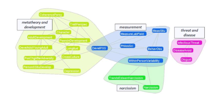
In the unsupervised approach, objectives include finding unknown patterns, developing a set of types (or a taxonomy), and assessing the dimensionality of a latent set of variables. In psychology, a focal problems involves assessing the factor structure of personality (if you have taken introductory psychology, you are likely familiar with the five-factor or Big Five model of personality). The unsupervised approach is also used to solve problems of community detection in the study of social and scientific networks (see Figure 20.1, from Lanning (2017)). I think that questions about dimensionality and internal structure can be compelling (Lanning 1994, 1996; Lanning and Rosenberg 2009), but I will not consider them further here.
21.2 prediction versus classification
Within the category of supervised problems, we can distinguish problems in classification (those in which the outcome is nominal or discrete) from problems where the outcome is ordered or numeric. We examined the Fair data in both these ways, first treating the outcome as the rescaled number of reported affairs, then as a distinction between those who did and did not have affairs.
Somewhere in between these two approaches are problems in which the criterion is an ordered set of categories - such as small, medium, and large pizza sizes or, to consider a problem in my own area of study, a sequence of seven levels of social maturity or personality development. Working with several colleagues, I constructed “dictionaries” which empirically distinguished these levels; the object is to allow assessment of the level of maturity or ego development of a given text. In the diagram below, the words in these initial dictionaries are arranged clockwise, with those characteristic of the earliest (Impulsive) level in the upper right quadrant (i.e., at 1 o’clock), then moving through the middle stages at the bottom, etc.(Lanning et al. (2018)). 
21.3 understanding versus prediction
In machine learning, we are in general concerned with the problem of finding the function which relates an outcome (Y) to a set of predictors (X). This general principle spans two opposing, but overlapping, use-cases: understanding and prediction.
For example, in the ‘Fair’ data, we were initially concerned with the question of “what predicts infidelity?,” which involves or suggests an interest in understanding. With the k-nn analysis, our focus increasingly shifted away from this towards the more pragmatic goal of increasing our hit rate or overall accuracy, away from a concern with inference and understanding to a position where we were satisfied to treat the algorithm as a black box from which we were only concerned with the accuracy of outputs.
These two objectives of “understanding and thinking in terms of equations and models” and “prediction and thinking only in terms of optimization” can be thought of as two points on a continuum of interpretability. Some techniques used in machine learning give results that are quite interpretable (including multiple regression, particularly restricted regression techniques such as the lasso). Others, including support vector machines and, in particular, deep neural networks sacrifice interpretability in the service of prediction. For complex approaches in image recognition, such as the chihuahua versus muffin problem, deep neural networks provide the best solutions, but are particularly challenging to understand (Kumar, Wong, and Taylor 2017).
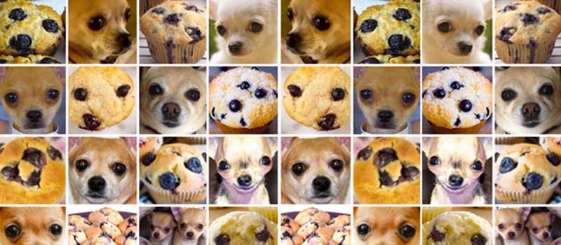
Fig 21.1: The chihuahua-muffin problem.
Exercise 21.1: Consider the Chihuahua-Muffin problem illustrated above.
What is the outcome variable ‘Y?’
What are some of the predictors ‘X?’ (Note that in image recognition and natural language processing, predictors are typically called “features”).
Why is this problem interesting? That is, are there problems similar to this that have important social uses?
Can you describe a simple algorithm or decision rule which works more than 50% of the time on the (training) data above (i.e., “if X then”Chihuahua" else “Muffin”)?
What might an effective algorithm on new (test) data look like?
finally, what do you think goes on on your mind as you evaluate the photos in the “chihuahua-muffin problem?”
21.4 bias versus variability
If you read further about machine learning, you are likely to encounter the phrase “bias-variability tradeoff.” You may remember that, in our initial analyses of the Swiss fertility data, we discussed how reducing the number of observations increases the fit of the model on the (training) data - and that, ultimately, the fit of the model would become perfect when we reduce the number of observations to the number of variables in the model.
Here, we construct two independent samples, each with 9 subjects.
data(Fair)
set.seed(33458)
FairSample1 <- Fair %>% sample_n(9)
set.seed(94611)
FairSample2 <- Fair %>% sample_n(9)
In the following chunk, we run a regression analysis witin each of these samples, predicting the number of affairs from the 9 predictors (including the intercept).
affairReg1 <- lm(nbaffairs ~ ., data=FairSample1)
affairReg2 <- lm(nbaffairs ~ ., data=FairSample2)

R21 <- summary(affairReg1)$r.squared
R22 <- summary(affairReg2)$r.squared
t(c(sample1 = R21, sample2 = R22)) %>%
kable(caption = "R^2 from two small samples")| sample1 | sample2 |
|---|---|
| 1 | 1 |
names(affairReg1[["coefficients"]]) %>%
    cbind(round(affairReg1[["coefficients"]], 2)) %>%
    cbind(round(affairReg2[["coefficients"]], 2)) %>%
    as_tibble() %>%
    rename(variable = 1,
           sample1 = 2,
           sample2 = 3) %>%
kable(caption = "Regression coefficients from two small samples") | variable | sample1 | sample2 |
|---|---|---|
| (Intercept) | 19.93 | 87.53 |
| sexmale | -3.7 | 49.39 |
| age | -0.16 | -2.96 |
| ym | 0.35 | 2.5 |
| childyes | 0.72 | -4.45 |
| religious | -0.79 | -4.55 |
| education | -0.49 | -0.88 |
| occupation | 2.33 | 2.95 |
| rate | -3.81 | -1.5 |
Note that in each case we have perfect predictability, but with a very different set of predictors. The difference between these two sets of coefficients is an illustration of how coefficients in overfit models will vary from one sample to another. At the opposite extreme are underfit models, which are likely to provide relatively stable coefficients across samples, but which aren’t very effective at prediction. This is the bias-variability trade-off, and it occurs not only in tiny data sets such as these, but in bigger datasets where there is a large number of predictor variables, as is often the case in, for example, artificial intelligence (including image recognition) and bioinformatics (including statistical genetics).
The problem of “too many predictors” can be addressed, in part, by “preprocessing,” or trying to restructure the data to effectively increase the number of rows in the data (e.g., by imputing missing values), or decrease the number of columns (that is, using component or factor analysis as an initial step in data analysis). Another approach is to use resampling.
21.4.1 resampling: beyond test, training, and validation samples
We’ve considered one approach to avoiding chance-inflated models and prediction estimates, and that is the approach of ‘holding out’ test (and possibly validation) samples. An extension of this approach is k-fold cross validation, in which the sample is divided into k (e.g., ten) parts, each of which is used as a validation sample in k different analyses. To assess the overall performance of the model, the results of these are averaged. This is a sophisticated and relatively easy to implement approach which can be used, for example, to assess the relative performance of different models, such as linear versus non-linear models.
Another approach to resampling is bootstrapping, in which model parameters (e.g., regression coefficients) are taken as the average of many (for example 1,000) analyses of subsamples of the data. In the bootstrap, sampling is done with replacement, so that the same case may appear in many samples. The averaged coefficients arrived at using bootstrapping are less variable than the results of a single analysis.
21.5 compensatory versus non-compensatory problems
Consider two simple hypothetical real world problems. In the first, you are deciding where you should apply to graduate school. Assume that, in the sample of schools under consideration, only two variables matter to you, say “program quality” and “program cost,” and that you weight the first of these positively and the second negatively. We might anticipate that these would be related in a compensatory way, so that you would be willing to pay more for a better program.
In the second problem, you are looking to hire a group of commercial jet pilots. Again, there are only two predictors; here, they are eyesight and responsibility. Unlike in the first problem, these are related in a noncompensatory way - for example, no matter how good someone’s eyesight is, if they are irresponsible you will not want to hire them. Similarly, even if they are very responsible, poor eyesight might make them ineligible.
Exercise 21.2: For the grad school and airline pilot problems, draw a pair of coordinate axes, together with points representing a few dozen “positive” (apply or hire) and “unacceptable” (don’t apply, don’t hire) observations. What can you say about the boundary between these two regions in each problem?
We can think of problems such as the grad school problem in a regression framework, while the pilot problem is instead a decision tree or “multiple cutoff” model. Very simple decision trees, including “fast and frugal trees,” can be useful tools both to describe how people decide and how they might make better decisions (Phillips et al. 2017).
In machine learning problems, there may be hundreds or thousands of predictors (features). The logic of decision trees is extended in techniques including bootstrap aggregation or bagging (in which a large number of trees are considered, then averaged), and random forests (which sequentially examines subsets of predictors in an effort to increase the reliability of predictions). These models are often predictively useful, but can be complex and difficult to interpret. Chapter 8 of (James et al. 2013) goes into more detail on these methods.
Two additional methods bear mention: Support vector machines (SVM) are classifiers which attempt to find optimal margins (hyperplanes) between two or more sets of criteria. Finally, neural networks are models which typically include multiple layers (akin to biological neurons) each of which can be activated based on the sum of the inputs of the prior layer. The chain of prediction from input (pixel) to output (“chihuahua”) is not a simple forward path, rather, errors of prediction are used to tune weights of intermediate layers in a process known as backpropagation. Artificial neural networks are, at present, the most important set of techniques in artificial intelligence problems including image, speech, and even taste recognition.
21.6 a postscript: The Tidymodels packages
The new Tidymodels packages provide a handful of new, tidyverse-compliant approaches to problems in prediction, modeling, and machine learning. The website, particularly the Get Started page, is straightforward, and I urge you to review it systematically. Here’s a quick summary of some key points from the first few pages of that section:
The parsnip package presents a tidyverse-compliant approach to writing syntax of models; it appears to be particularly useful for examining multiple models on the same data sets.
The broom package includes the tidy() function, which can be used to present the results of your analyses in data frames - this is handy for making tables of your data. Results of these models can be represented as data frames, which can then be easily tabled or used to create figures. You can see how these are used on the Build a model page.
Perhaps the most useful tool introduced in these pages is the Skimr package. Skimr, though not part of the Tidymodels, is handy for getting a quick set of summary statistics - it’s substantially more convenient than the summarise function in the Tidyverse and, unlike the describe package in the psych package, is Tidyverse-compliant.
The preprocessing of data includes several concepts that we have previously considered, including splitting data into training and test subsamples, the creation of dummy variables, and how we can treat time data. The recipes package include several functions that make it more convenient to work with only subsets of our variables, that is, to assign “roles” to include or exclude variables in our models. This section also includes an introduction to the yardstick package, which gives an easier way to implement ROC analysis than the code I used in the prior chapters.
Resampling is a process through which we can estimate model parameters by inspecting a series of subsets of the data. It is particularly useful when we want to compare a set of competing models on a small-ish dataset (Lanning et al. 2018). This section also includes an application of the random forests model introduced above.